About
Best Practice Guide on establishing nutrient concentrations to support good ecological status
Geoff Phillips, Martyn Kelly, Wera Leujak, Fuensanta Salas, Heliana Teixeira, Anne Lyche Solheim, Gary Free, Gabor Varbiro
Final version following testing at Bucharest workshop November 2018
Summary
- 1. High concentrations of inorganic nutrients are a major factor contributing to the failure of many water bodies to achieve Good Ecological Status and Member States need to determine levels appropriate to their own territories.
- 2. This report describes statistical methods for determining appropriate concentrations for supporting ecological status. These statistical methods need to be set in a broader framework that also encompasses chemical, ecological and regulatory aspects relevant to the type of water body under consideration.
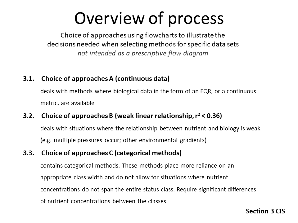
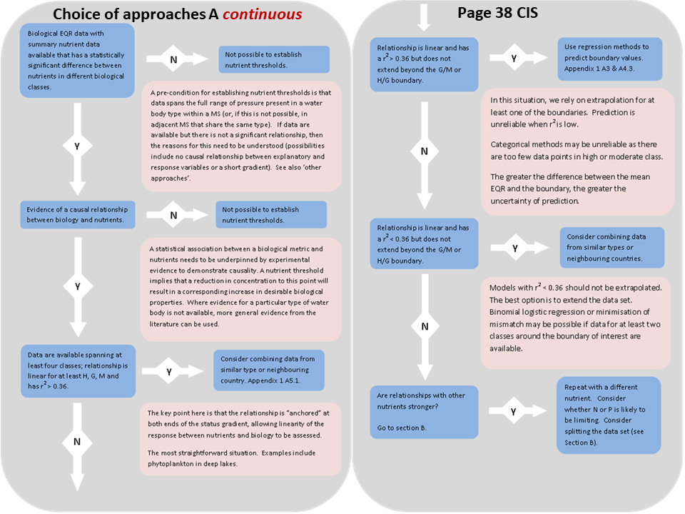
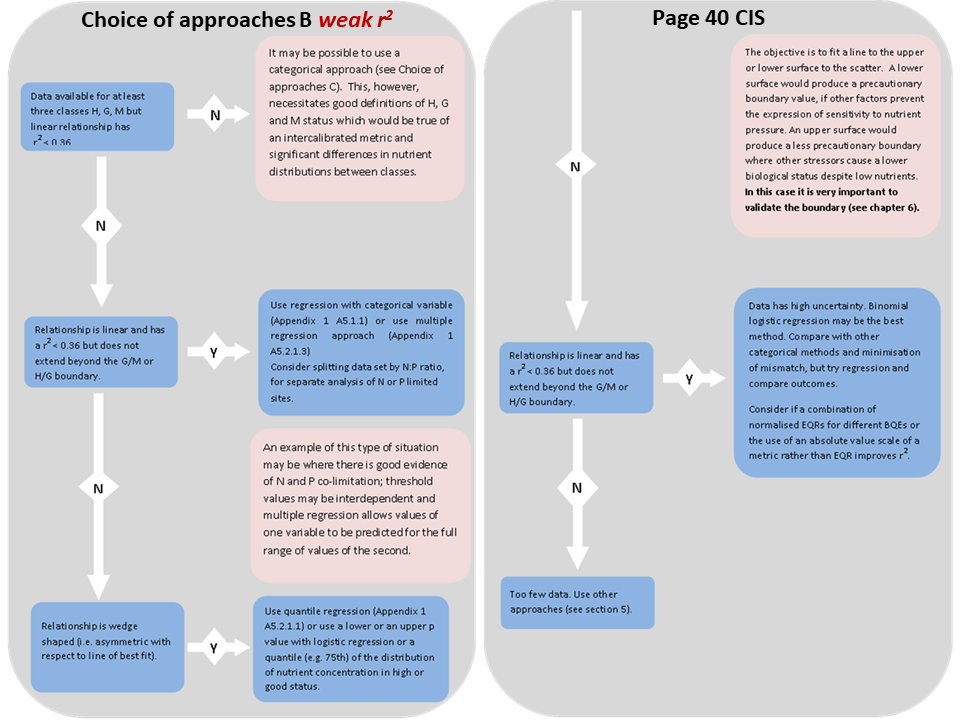
- 3. Three approaches to setting these threshold concentrations are included. These are: • Regression analysis, using a continuous relationship between EQR and nutrient concentration • Categorical analysis, using the distribution of nutrient concentration within biological classes • Minimisation of mis-match of classifications for biology and nutrients
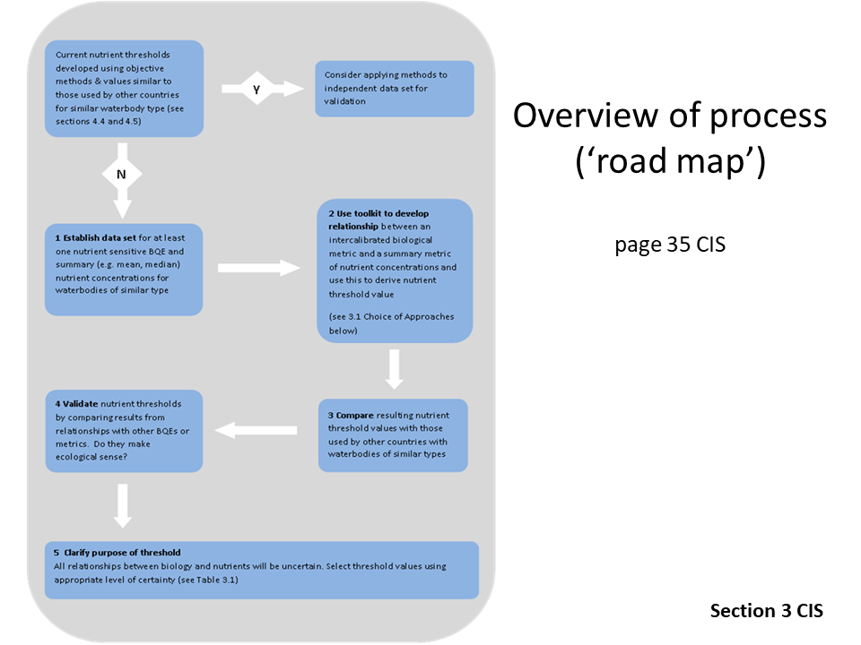
- 4. The choice of method depends upon a number of factors, including the length of the gradient that available datasets cover and the statistical strength of the relationship between the explanatory and response variables. In some cases, Member States may be better able to achieve the statistical prerequisites for methods by joining forces with neighbours who share similar water body types.
- 5. Excel and R-based statistical “toolkits” are provided in order to make calculation of threshold concentrations more straightforward.
- 6. Options for situations where none of these methods are appropriate are also described.
- 7. Finally, some practical issues associated with the use of these threshold concentrations for regulation are discussed.
Disclaimer
This application has been developed through a collaborative framework (the Common Implementation Strategy (CIS)) involving the Member States, EFTA countries, and other stakeholders including the European Commission. The document is a working draft and does not necessarily represent the official, formal position of any of the partners.
To the extent that the European Commission's services provided input to this technical document, such input does not necessarily reflect the views of the European Commission.
Neither the European Commission nor any other CIS partners are responsible for the use that any third party might make of the information contained in this document.
The technical document is intended to facilitate the implementation of Directive 2000/60/EC and is not legally binding. Any authoritative reading of the law should only be derived from Directive 2000/60/EC itself and other applicable legal texts or principles. Only the Court of Justice of the European Union is competent to authoritatively interpret Union legislation.
Reference
Please reference the use of this application in any publications as
Gabor Varbiro, Heliana Teixeira, Martyn Kelly and Geoff Phillips (2018)A Shiny application of a statistical toolkit to assist with the development of nutrient concentrations that would support good ecological status for the Water Framework Directive.
Import
Select the proper separator and decimal settings before loading the data
*In order to test the application ....
You can download an empty Data Template here :
DataTemplate.csvContent
Summary
Names
Focus
Plot_EQR Outliers
Before proceeding with the Toolkit you can select outliers to exlude from the analyses (Red dots). Blue dots : sample points, Black dots: samples with Exclude mark in the uploaded file
* the black dots doesn't excluded by default, you should click on them...
Plot Ouddtliers
Scatterplot of Nutrient vs. EQR for water bodies colored by groups
Scatterplot of Nutrient vs. EQR for water bodies colored by groups
Plot P by EQR classes
Figure A-8 Range of Nutrient concentrations for water bodies grouped by quality class
Plot 2nd Nutrient by EQR classes
Figure A-8 Range of TN concentrations for water bodies grouped by quality class
Plot Nutrient by EQR Classes
Figure A-8 Range of TP concentrations for water bodies grouped by predifined quality class
Plot Nutrient by EQR Classes
Figure A-8 Range of TN concentrations for water bodies grouped by predifined quality class
Plot Nutrient by Groups
Plot Nutrient by Groups
Plot_EQR vs Nutrient
Plot_EQR vs Nutrient Quantile regression
Figure Scatterplot of TP vs. EQR the quantile regression lines coresspond to the 5, 25, 50, 75 and 95 quantiles.
Plot_EQR vs Nutrient
Plot_EQR vs Nutrient Quantile regression
Figure Scatterplot of TN vs. EQR the quantile regression lines coresspond to the , 25, 50, 75 and 95 quantiles.
Adjust Nutrient range
The toolkit allows three regression models to be fitted to the linear portion of the data:
- an Ordinary Least Squares (OLS) regression of EQR v nutrient concentration; assumes all uncertainty is in measurement of the EQR (underestimate of slope);
- an OLS regression of nutrient v EQR; assumes all uncertainty lies in measurement of nutrient concentrations (overestimate of slope);
- a type II regression; assumes equal uncertainty in measurement of both EQR and nutrient (slope between the two OLS regressions).
The boundary values predicted by the regression models depend on the slope of the relationship and the difference in the slopes produced by these relationships depends on the r2 : the lower the value the greater the difference.
It is important to stress that selecting the segment of data to be used will have a significant influence on the slope of the linear models and thus the predicted boundary values and is to an extent a subjective decision, albeit guided by the gam and segmented regression models.
Segmented regression
To fit a segmented regression, it is necessary to estimate the break points. In the test data set curvature is not that marked, thus it is best to start with a single break point. Other data sets may clearly require two break points and to accommodate these two different functions have been provided
For one break points
For two break points
OLS Regression of EQR on Nutrient
Figure A-14 Relationship between EQR and Nutrient concentration in test data set showing OLS regression of EQR vs Nutrient. Predicted good/moderate boundary values shown.
OLS Regression of Nutrient on EQR
Figure A-14 Relationship between EQR and Nutrient concentration in test data set showing OLS regression of Nutrient on EQR (inverted to plot on same scales). Predicted good/moderate boundary values shown.
Ranged major axis regression EQR vs. Nutrient
Figure A-14 Relationship between EQR and Nutrient concentration in test data set showing RMA type II regression. Predicted good/moderate boundary values shown.
Linear methods results
Data.frame contains the following values as columns: Model, r2, the number of observations used N, slope, intercept, predicted good/moderate boundary GM, lower and upper estimates of good/moderate boundaries GML GMU, the high/good boundary HG, lower and upper estimates of high/good boundaries HGL HGU. Rows are results for Model 1, Model 3 and Model 2.
High-Good mis-match plot
Good-Moderate mis-match plot
Boxplot methods results
Boxplot summary table
Boxplot summary
If the differences between the nutrient concentrations in adjacent classes are not significant, treat quantiles with extreme caution
Wilcox test the differences between the nutrient concentrations
Quantile regression results
Linear quantiles
Figure: Scatterplot of Nutrient vs. EQR the quantile regression lines coresspond to the 25th(red), 50th(black) and 75th quantiles(blue).
* The linear quantiles restricted for the data range choosen with the range sliders in the linear methodsQuantile table
Additive quantiles
* The Additive quantiles cover the full data range Note how the additive model is significantly influenced where the number of data points are low at the ends of the axes. A linear quantile model fitted to a sub-set of the data may be more usefulHigh-Good bootstrap mis-match plot
Figure A-25 Relationship between percentage of mis-classified records comparing biological and nutrient classifications in comparison to value of nutrient boundary. Vertical lines mark the range of cross-over points where the mis-classification is minimized, together with the mean nutrient concentration. (each line shows a sub-sample of the data set selected at random)
Range of cross-over values
Range of percentage mis-match at cross-over
Good-Moderate bootstrap mis-match plot
Figure A-25 Relationship between percentage of mis-classified records comparing biological and nutrient classifications in comparison to value of nutrient boundary. Vertical lines mark the range of cross-over points where the mis-classification is minimized, together with the mean nutrient concentration. (each line shows a sub-sample of the data set selected at random)
Range of cross-over values
Range of percentage mis-match at cross-over
Best Practice Guide How-to
First Import the file or use the sample dataset. Don't forget to use the proper decimal and separation symbols.
The content of the data / boxplots etc can be found in the Check data tab
You can adjust the EQR boundaries, the application recalculate all statistic with the new values
You can set the focus of the analysis to TP or TN the application recalculate all statistic with the new values
Before proceeding with the Toolkit you can select outliers to exlude from the analyses
You can adjust the Nutrient boundaries for linear and mismatch methods check the R2 to achieve the best correlation, the application recalculate all statistic with the new values.
Best Practice Guide Analyses guides
Logistic method result
Logistic plot
Figure A-27 Binomial logistic regression of the Nutrient on probability of being good or worse status. Lines show potential boundary values at different probabilities of being good or worse. Grey areas shows uncertainty band ± SE
Figure A-27 Binomial logistic regression of the Nutrient on probability of being moderate or worse status. Lines show potential boundary values at different probabilities of being moderate or worse. Grey areas shows uncertainty band ± SE
Set molar N:P ratio for Coplots
Calculate molar N:P ratio, Use the appropriate setting for the used factor
Phosphorus as variable conditioned by Nitrogen
Coplot P as variable conditioned by N
Figure A-10 Relationship between EQR for biological element and total phosphorus (log10) for different ranges of total nitrogen concentration
Phosphorus as variable conditioned by NP ratio
Coplot P as variable conditioned by NP ratio
Figure A-11 Relationship between EQR for biological element and total phosphorus (log10) for different ranges of the N:P ratio
Nitrogen as variable conditioned by Phosphorus
Coplot N as variable conditioned by P
Figure A-10 Relationship between EQR for biological element and total nitrogene (log10) for different ranges of total phosphorus concentration
Nitrogen as variable conditioned by NP ratio
Coplot N as variable conditioned by NP ratio
Figure A-11 Relationship between EQR for biological element and total nitrogene (log10) for different ranges of the N:P ratio
Multiple regression results
Multiple methods results
Figure 1a Relationship between mean TN and TP. Points coloured by biological class, dotted line marks the mean N:P ratio, green lines show contours that would predict the good/moderate EQR boundary of 0.6 (dotted green lines show uncertainty band). Horizontal and vertical dotted lines show potential pairs of TN and TP boundaries together with their uncertainty ranges.
Figure 1b Relationship between mean TN and TP. Points coloured by biological class, dotted line marks the mean N:P ratio, blue lines show contours that would predict the high/good EQR boundary of 0.6 (dotted blue lines show uncertainty band). Horizontal and vertical dotted lines show potential pairs of TN and TP boundaries together with their uncertainty ranges.